Copy And Paste Formulas As Values. After using the Excel formulas to change the case of our text, we may want to convert these to values. This can be done by copying the range of formulas and pasting them as values with the paste special command. If you miss it, Excel will mistake your formula as regular text. Space before equal sign: You are not supposed to enter any space before equal sign. Maybe a single space will be hard for us to detect, but it breaks the rule of writing formulas for Excel. Formula wrapped in quotes: You need to make sure that your formula is not wrapped in quotes. CUBEVALUE – This formula will calculate a value directly from the data cube based on parameters that passed into the formula, including cube members or slicer values. CUBESET – This formula extracts all unique values from a set expression, and can apply a sort based on. Normally this will be a single table column when working with the. To copy the actual value instead of the formula from the cell to another worksheet or workbook, you can convert the formula in its cell to its value by doing the following: Press F2 to edit the cell. Press F9, and then press ENTER. After you convert the cell from a formula to a value, the value appears as 1932.322 in the formula bar. Boolean Values and Excel Formulas. Unlike arithmetic functions, formulas in Excel and Google Sheets that carry out arithmetic operations such as addition and subtraction are happy to read Boolean values as numbers without the need for conversion. Such formulas automatically set TRUE equal to 1 and FALSE equal to 0.
The present value calculations on this page are applied to investments for which interest is compounded in each period of the investment.
However if you are supplied with a stated annual interest rate, and told that the interest is compounded monthly, you will need to convert the annual interest rate to a monthly interest rate and the number of periods into months:
| monthly interest rate | = | annual interest rate / 12 |
| number of months | = | number of years * 12 |
A similar conversion is required if interest is paid quarterly, semi-annually, etc.
For an example of this, see the section on How To Calculate Present Value When Interest is Compounded Monthly
Present Value Index:
| Present Value of a Single Cash Flow |
| Present Value of a Series of Cash Flows |
| Present Value of a Perpetuity |
Present Value of a Single Cash Flow
If you want to calculate the present value of a single investment that earns a fixed interest rate, compounded over a specified number of periods, the formula for this is:
where,
- fv is the future value of the investment;
- rate is the interest rate per period (as a decimal or a percentage);
- nper is the number of periods over which the investment is made.
| A | B | |
|---|---|---|
| 1 | Future Value: | 15000 |
| 2 | Annual Interest Rate: | 4% |
| 3 | Number of Years: | 5 |
| 4 | Present Value: | =15000/(1+4%)^5 |
For example, if you want a future value of $15,000 in 5 years' time from an investment which earns an annual interest rate of 4%, the present value of this investment (i.e. the amount you will need to invest) can be calculated by typing the following formula into any Excel cell:
which gives the result 12328.9066.
I.e. the present value of the investment (rounded to 2 decimal places) is $12,328.91.
As with all Excel formulas, instead of typing the numbers directly into the present value formula, you can use references to cells containing values. Therefore, the present value formula in cell B4 of the above spreadsheet could be entered as:
which returns the same result.
Using the Excel PV Function to Calculate the Present Value of a Single Cash Flow
Instead of using the above formula, the present value of a single cash flow can be calculated using the built-in Excel PV function (which is generally used for a series of cash flows).
The syntax of the PV function is:
where,
- rate is the interest rate per period (as a decimal or a percentage);
- nper is the number of periods over which the investment is made;
- [pmt] is the regular payment per period (if omitted, this is set to the default value 0);
- [fv] is the future value of the investment, at the end of nper payments (if omitted, this is set to the default value 0);
- [type] specifies whether the payment is made at the start or the end of the period.
This can have the value 0 or 1, meaning:
0 - the payment is made at the end of the period (as for an ordinary annuity);
1 - the payment is made at the start of the period (as for an annuity due).If omitted, the [type] argument is set to the default value 0.
Note that, in line with the general cash flow sign convention, the PV function treats negative values as outflows and positive values as inflows.
| A | B | |
|---|---|---|
| 1 | Future Value: | 15000 |
| 2 | Annual Interest Rate: | 4% |
| 3 | Number of Years: | 5 |
| 4 | Present Value: | =PV( 4%, 5, 0, 15000 ) |
For example, the above spreadsheet on the right shows the Excel PV function used to calculate the present value of an investment that earns an annual interest rate of 4% and has a future value of $15,000 after 5 years.
As shown in cell B4 of the spreadsheet, the PV function to calculate this is:
which gives the result -$12,328.91.
Note that in the above PV function:
- The [pmt] argument is set to 0, as there are no ongoing payments after the initial investment;
- The returned present value is negative, representing an outgoing payment.
How To Calculate Present Value When Interest is Compounded Monthly
If the interest on your investment is compounded monthly (while being quoted as an annual interest rate), the annual interest rate needs to be converted into a monthly interest rate and the number of years needs to be converted into months.
I.e.
| monthly interest rate | = | annual interest rate / 12 |
| number of months | = | number of years * 12 |
| A | B | |
|---|---|---|
| 1 | Future Value: | 15000 |
| 2 | Annual Interest Rate: | 4% |
| 3 | Number of Years: | 5 |
| 4 | Present Value: | =PV( 4%/12, 5*12, 0, 15000 ) |
Therefore, if an investment has a stated annual interest rate of 4% (compounded monthly), and returns $15,000 after 5 years, the present value of the investment can be calculated as follows:
which returns the result -$12,285.05.
(Note that, once again, the value returned from the PV function is negative, representing an outgoing payment).
Present Value of a Series of Cash Flows (An Annuity)
If you want to calculate the present value of an annuity (a series of periodic constant cash flows that earn a fixed interest rate over a specified number of periods), this can be done using the Excel PV function.
The syntax of the PV function is:
Converting Formulas To Values In Excel
where,
- rate is the interest rate per period (as a decimal or a percentage);
- nper is the number of periods over which the investment is made;
- [pmt] is the regular payment per period (if omitted, this is set to the default value 0);
- [fv] is the future value of the investment, at the end of nper payments (if omitted, this is set to the default value 0);
- [type] specifies whether the payment is made at the start or the end of the period.
This can have the value 0 or 1, meaning:
0 - the payment is made at the end of the period (as for an ordinary annuity);
1 - the payment is made at the start of the period (as for an annuity due).If omitted, the [type] argument is set to the default value 0.
Note that, in line with the general cash flow sign convention, the PV function treats negative values as outflows and positive values as inflows.
| A | B | |
|---|---|---|
| 1 | Annual Interest Rate: | 4% |
| 2 | Number of Years: | 5 |
| 3 | Annual Payment: | 500 |
| 4 | Present Value: | =PV( 4%, 5, 500 ) |
For example, to calculate the present value of an ordinary annuity that has an annual interest rate of 4% and returns payments of $500 per year for 5 years, type the following formula into any Excel cell:
which gives the result -$2,225.91.
Note that in the above PV function:
- The [fv] argument is omitted, and so takes on the default value 0;
- the [type] argument is omitted, and so takes on the default value 0 (i.e. the calculation assumes that the payment is made at the end of each year);
- The returned present value is negative, representing an outgoing payment.
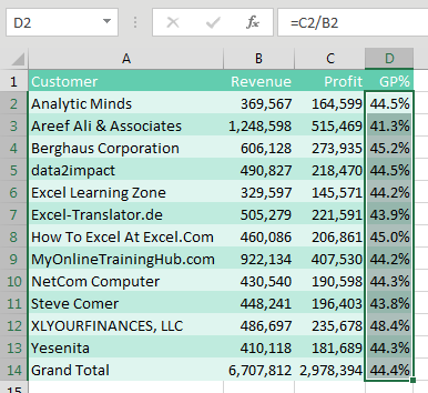
Convert Formula To Value In Excel 2007
Again, as with all Excel formulas, instead of typing the numbers directly into the present value formula, you can use references to cells containing values. Therefore, the PV function in cell B4 of the above spreadsheet could be entered as:
which returns the same result.
Present Value of a Perpetuity
A perpetuity is an annuity in which the constant periodic payments continue indefinitely.
The formula to calculate the present value of a perpetuity is:
where,
- pmt is the regular payment per period;
- rate is the interest rate per period (as a decimal or a percentage).
| A | B | |
|---|---|---|
| 1 | Annual Payment: | 30000 |
| 2 | Annual Interest Rate: | 3.5% |
| 3 | Present Value: | =30000/3.5% |
For example, if you have a perpetuity that pays $30,000 per year and has an annual interest rate of 3.5%, the present value of the perpetuity can be calculated by typing the following formula into any Excel cell:
This gives the result 857142.8571.
I.e. the present value of the perpetuity (rounded to 2 decimal places) is $857,142.86.
Return to the ExcelFunctions.net Home Page